 |
| 
Focusing and Collimating
Focusing and Collimating
Application 1: Focusing a Collimated Laser Beam
As a first example, we look at a common application, the focusing of a laser beam to a small spot. The situation is shown in Figure 5. Here we have a laser beam, with radius y1 and divergence θ1 that is focused by a lens of focal length f. From the figure, we have θ2 = y1/f. The optical invariant then tells us that we must have y2 = θ1f, because the product of radius and divergence angle must be constant.
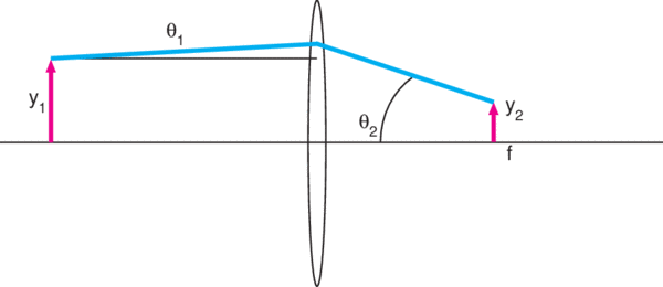
Figure 5
As a numerical example, let’s look at the case of the output from a Newport R-31005 HeNe laser focused to a spot using a KPX043 Plano-Convex Lens. This Hene laser has a beam diameter of 0.63 mm and a divergence of 1.3 mrad. Note that these are beam diameter and full divergence, so in the notation of our figure, y1 = 0.315 mm and θ1 = 0.65 mrad. The KPX043 lens has a focal length of 25.4 mm. Thus, at the focused spot, we have a radius θ1f = 16.5 µm. So, the diameter of the spot will be 33 µm.
This is a fundamental limitation on the minimum size of the focused spot in this application. We have already assumed a perfect, aberration-free lens. No improvement of the lens can yield any improvement in the spot size. The only way to make the spot size smaller is to use a lens of shorter focal length or expand the beam. If this is not possible because of a limitation in the geometry of the optical system, then this spot size is the smallest that could be achieved. In addition, diffraction may limit the spot to an even larger size (see Gaussian Beam Optics), but we are ignoring wave optics and only considering ray optics here.
Application 2: Collimating Light from a Point Source
Another common application is the collimation of light from a very small source, as shown in Figure 6. The problem is often stated in terms of collimating the output from a “point source.” Unfortunately, nothing is ever a true point source and the size of the source must be included in any calculation. In figure 6, the point source has a radius of y1 and has a maximum ray of angle θ1. If we collimate the output from this source using a lens with focal length f, then the result will be a beam with a radius y2 = θ1f and divergence angle θ2 = y1/f. Note that, no matter what lens is used, the beam radius and beam divergence have a reciprocal relation. For example, to improve the collimation by a factor of two, you need to increase the beam diameter by a factor of two.
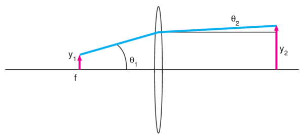
Figure 6
Since a common application is the collimation of the output from an Optical Fiber, let’s use that for our numerical example. The Newport F-MBB fiber has a core diameter of 200 µm and a numerical aperture (NA) of 0.37. The radius y1 of our source is then 100 µm. NA is defined in terms of the half-angle accepted by the fiber, so θ1 = 0.37. If we again use the KPX043 , 25.4 mm focal length lens to collimate the output, we will have a beam with a radius of 9.4 mm and a half-angle divergence of 4 mrad. We are locked into a particular relation between the size and divergence of the beam. If we want a smaller beam, we must settle for a larger divergence. If we want the beam to remain collimated over a large distance, then we must accept a larger beam diameter in order to achieve this.
Application 3: Expanding a Laser Beam
It is often desirable to expand a laser beam. At least two lenses are necessary to accomplish this. In Figure 7, a laser beam of radius y1 and divergence θ1 is expanded by a negative lens with focal length −f1. From Applications 1 and 2 we know θ2 = y1/|−f1|, and the optical invariant tells us that the radius of the virtual image formed by this lens is y2 = θ1|−f1|. This image is at the focal point of the lens, s2 = −f1, because a well-collimated laser yields s1 ~ ∞, so from the Gaussian lens equation s2 = f. Adding a second lens with a positive focal length f2 and separating the two lenses by the sum of the two focal lengths −f1 +f2, results in a beam with a radius y3 = θ2f2 and divergence angle θ3 = y2/f2.
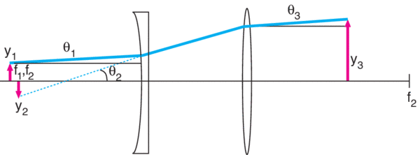
Figure 7
The expansion ratio
y3/y1 = θ2f2/θ2|−f1| = f2/| −f1|
or the ratio of the focal lengths of the lenses. The expanded beam diameter
2y3 = 2θ2f2 = 2y1f2/|−f1|
The divergence angle of the resulting expanded beam
θ3 = y2/f2 = θ1|−f1|/f2
is reduced from the original divergence by a factor that is equal to the ratio of the focal lengths |-f1|/f2. So, to expand a laser beam by a factor of five we would select two lenses whose focal lengths differ by a factor of five, and the divergence angle of the expanded beam would be 1/5th the original divergence angle.
As an example, consider a Newport R-31005 HeNe Laser with beam diameter 0.63 mm and a divergence of 1.3 mrad. Note that these are beam diameter and full divergence, so in the notation of our figure, y1 = 0.315 mm and θ1 = 0.65 mrad. To expand this beam ten times while reducing the divergence by a factor of ten, we could select a plano-concave lens KPC043 with f1 = -25 mm and a plano-convex lens KPX109 with f2 = 250 mm. Since real lenses differ in some degree from thin lenses, the spacing between the pair of lenses is actually the sum of the back focal lengths BFL1 + BFL2 = -26.64 mm + 247.61 mm = 220.97 mm. The expanded beam diameter
2y3 = 2y1f2/|-f1| = 2(0.315 mm)(250 mm)/|-25 mm|= 6.3 mm.
The divergence angle
θ3 = θ1|-f1|/f2 = (0.65 mrad)|-25 mm|/250 mm = 0.065 mrad.
For minimal aberrations, it is best to use a plano-concave lens for the negative lens and a plano-convex lens for the positive lens with the plano surfaces facing each other. To further reduce aberrations, only the central portion of the lens should be illuminated, so choosing oversized lenses is often a good idea. This style of beam expander is called Galilean. Two positive lenses can also be used in a Keplerian beam expander design, but this configuration is longer than the Galilean design.
Application 4: Focusing an Extended Source to a Small Spot
This application is one that will be approached as an imaging problem as opposed to the focusing and collimation problems of the previous applications. An example might be a situation where a fluorescing sample must be imaged with a CCD camera. The geometry of the application is shown in Figure 8. An extended source with a radius of y1 is located at a distance s1 from a lens of focal length f. The figure shows a ray incident upon the lens at a radius of R. We can take this radius R to be the maximal allowed ray, or clear aperture, of the lens.
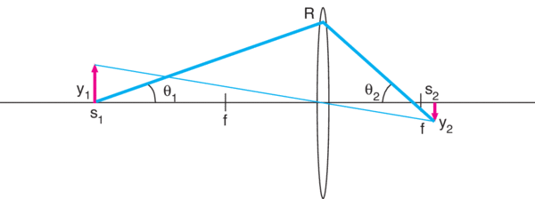
Figure 8
If s1 is large, then s2 will be close to f, from our Gaussian lens equation, so for the purposes of approximation we can take θ2 ~ R/f. Then from the optical invariant, we have
y2 = y1θ1/θ2 = y1(R/s1)(f/R) or y2 = 2y1(R/s1)f/#
where f/2R = f/D is the f-number, f/#, of the lens. In order to make the image size smaller, we could make f/# smaller, but we are limited to f/# = 1 or so. That leaves us with the choice of decreasing R (smaller lens or aperture stop in front of the lens) or increasing s1. However, if we do either of those, it will restrict the light gathered by the lens. If we either decrease R by a factor of two or increase s1 by a factor of two, it would decrease the total light focused at s2 by a factor of four due to the restriction of the solid angle subtended by the lens.